Date: May, 2022
So far in this class, I have implemented PID feedback control, mapping, and localization algorithms. The goal of this lab was to use whatever pieces of knowledge and the skills learned in this class to get the real robot to visit 9 set waypoints marked in the map.
First Attempt: Dead Reckoning
Towards the beginning of this class we talked about dead reckoning in lecture. Dead reckoning is the process of estimating your current position by using previous position data and incorporating velocity and/or angular orientation data over time. Therefore, the IMU sensor is potentially a good tool to perform dead reckoning. I wanted to try to use dead reckoning with the accelerometer even though in class we talked about its drawbacks, because we hadn’t implemented it in class yet. Dead reckoning is extremely susceptible to accumulation errors especially with a noisy sensor like the accelerometer. I definitely saw this issue pop up and it was ultimately the reason I decided to move onto a new method for executing the path.
My original idea was to use PID feedback control on the orientation for making turns and ensuring I was driving in a straight line (not drifting). Since the robot would be moving in a straight line, I thought doing dead reckoning would have less issues with accuracy than doing dead reckoning along a curved path.
The following are parts of the code I wrote to compute the dead reckoning. I integrate the acceleration to get the velocity and then integrate the velocity to get the position. I also implemented a low pass filter on the acceleration. I put a lot more trust in the previous accelertaion data point as you can see by the constant a = 0.15.
double acc_LPF[] = {0, 0};
double vel[] = {0, 0};
double pos[] = {0, 0};
const int n = 1;


dt = (micros() - prev_t) / 1000000.0;
prev_t = micros();


acc = (myICM.accX() / 1000 * 9.807); //convert units from mg > g > m/s^2

// Low Pass Filter Accelertation
const float a = 0.15;
acc_LPF[n] = a * acc + (1 - a) * acc_LPF[n - 1];

// Velocity
vel[n] = vel[n - 1] + acc_LPF[n - 1] * dt;

// Distance/Position
pos[n] = pos[n - 1] + vel[n - 1] * dt;

// Update
acc_LPF[n - 1] = acc_LPF[n];
vel[n - 1] = vel[n];
pos[n - 1] = pos[n];
The blue curve is acceleration, the red curve is velocity, and the greed curve is position. The velocity and position curves are in units of cm/s and cm for ease of visualization. The acceleration is in m/s^2.
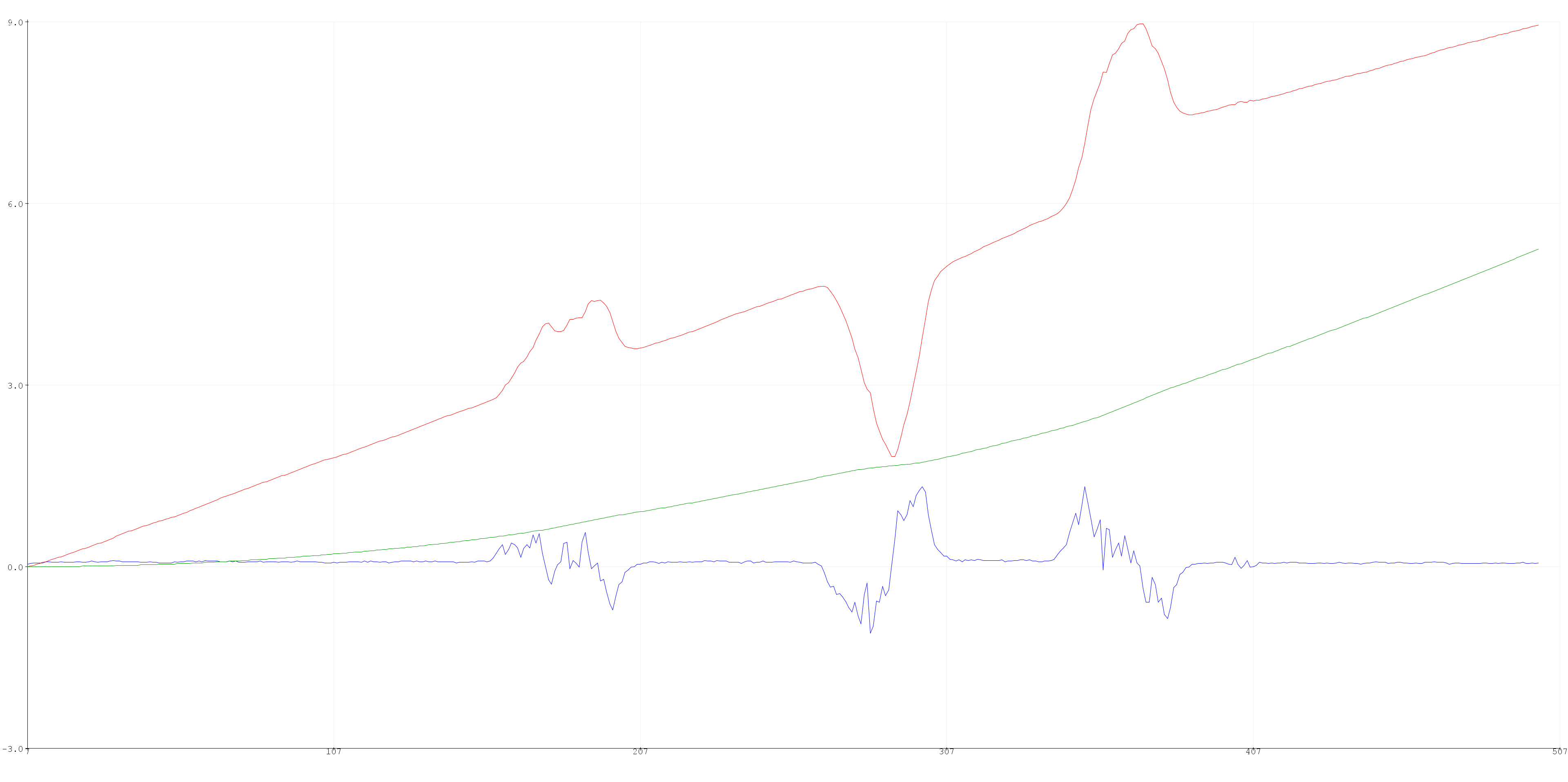
I pushed the robot forward once, pulled the robot backwards once, and then pushed the robot forward again. You can see the 3 bumps in the velocity data and the corresponding changes in the acceleration data.
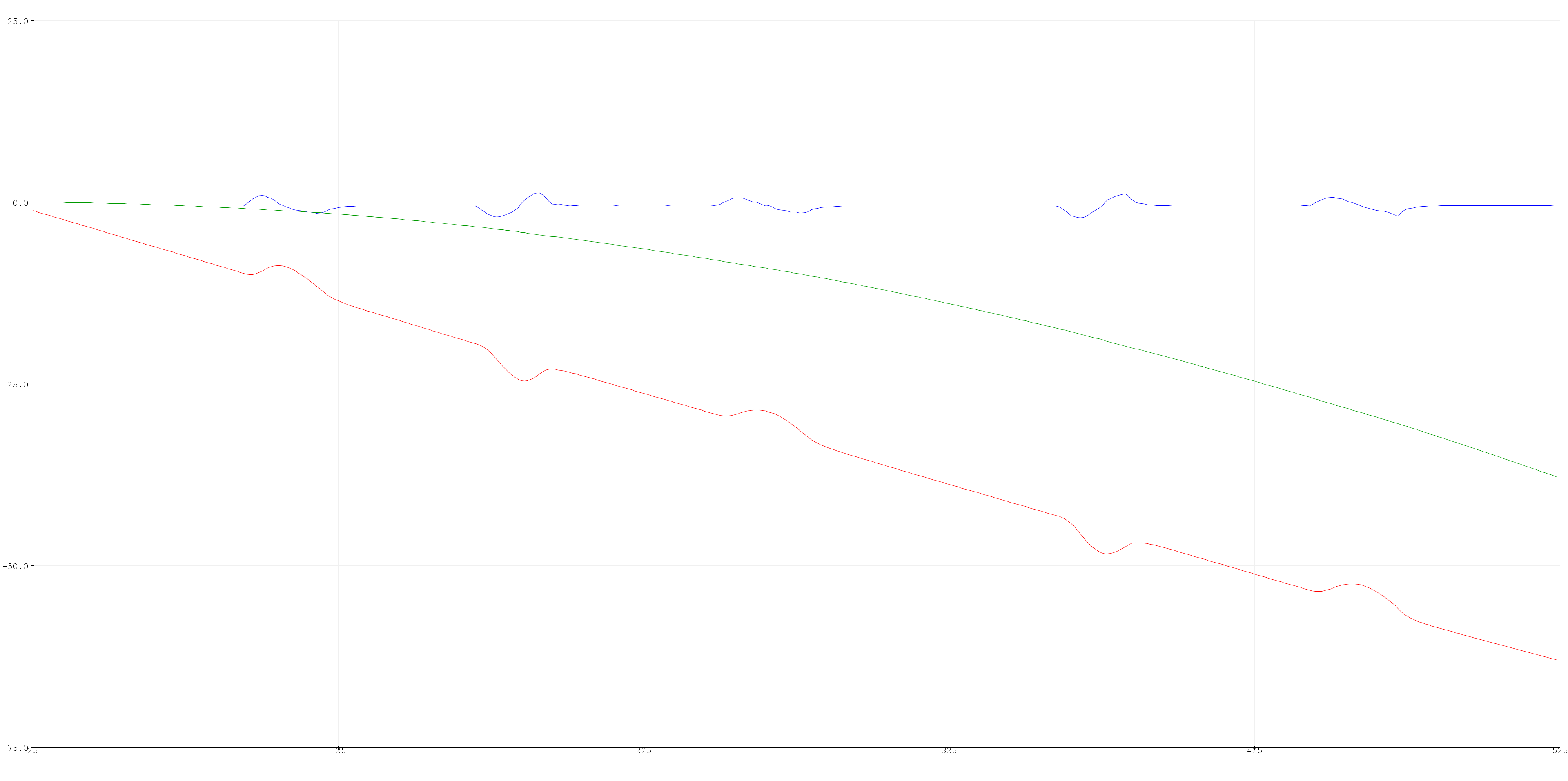
I was still facing issues with the data, so I set up the sensor’s built-in digital low pass filter to see if that would improve the data. I messed abournd with some of the settings and saw some improvemnts in the acceleration data but nothing too significant. The acceleration curves look smoother, but the velocity curve (and postion curve) are still accumulating a lot of error.
ICM_20948_dlpcfg_t myDLPcfg;    // Configuration structure for the desired sensors (accel & gyro)

myDLPcfg.a = acc_d111bw4_n136bw; // (ICM_20948_ACCEL_CONFIG_DLPCFG_e)
myDLPcfg.g = gyr_d361bw4_n376bw5; // (ICM_20948_GYRO_CONFIG_1_DLPCFG_e)

myICM.setDLPFcfg((ICM_20948_Internal_Acc | ICM_20948_Internal_Gyr), myDLPcfg);

// Choose whether or not to use DLPF
ICM_20948_Status_e accDLPEnableStat = myICM.enableDLPF(ICM_20948_Internal_Acc, true);
ICM_20948_Status_e gyrDLPEnableStat = myICM.enableDLPF(ICM_20948_Internal_Gyr, true);
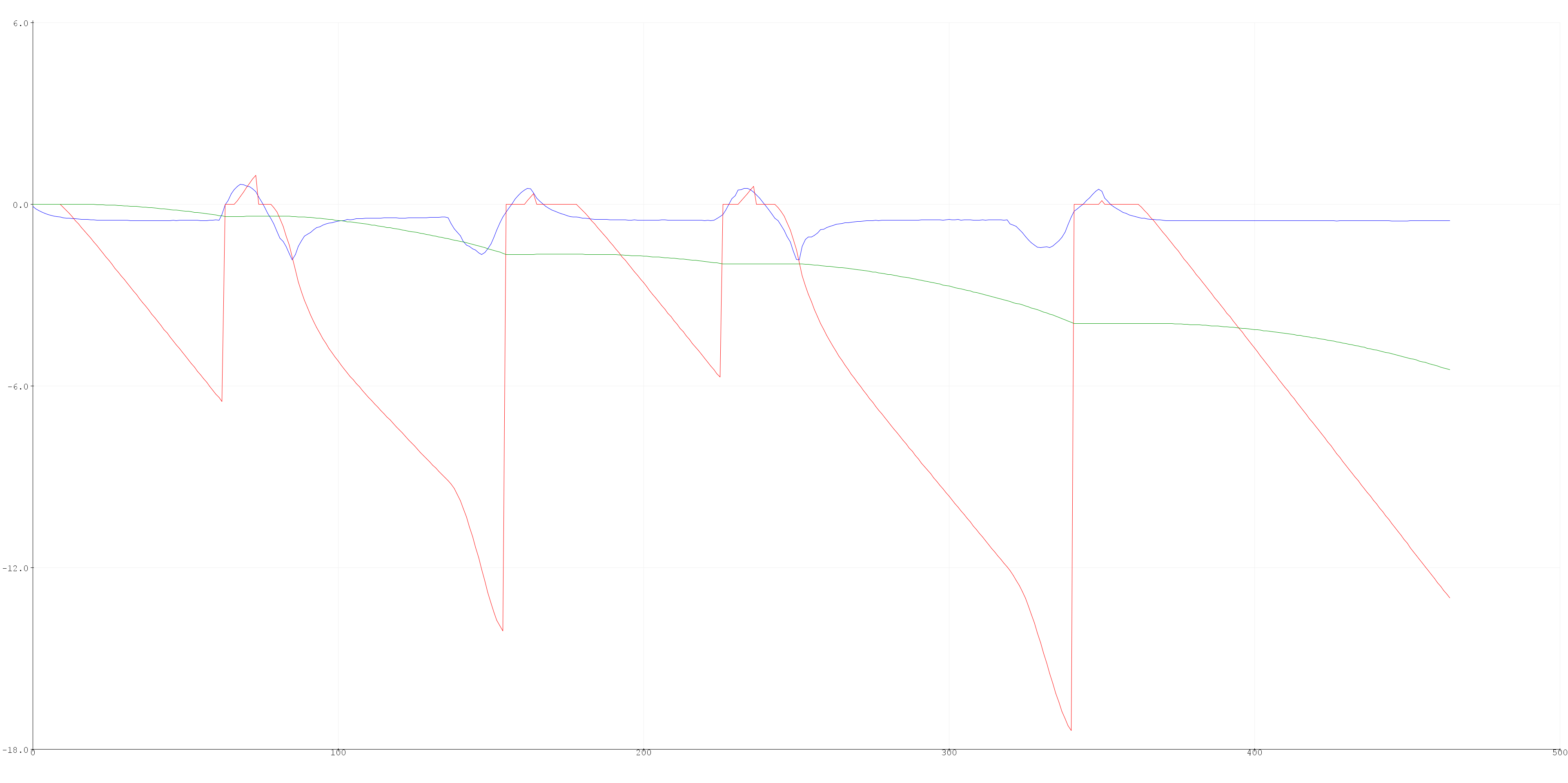
Another fix I tried was to just get rid of the steadily increasing part of the velocity curve. You can see the bumps in the previous two graph were I move the robot, when it did have some non-zero velocity. I estimated the slope of the non-peaked portions of the graph. If the change in velocity was less than or equivalent to the slope, I set the velocity equal to zero.
if ( abs(vel[n] - vel[n - 1]) <= 0.001) {
  vel[n] = 0;
}
This didn’t end up working as intended. When the acceleration starts to decrease (at the peak of the velocity bumps), the velocity is small enough to be in the range of the magnitude of the slope. This causes weird behaviors in the velocity and position curves.
Ultimately, I could not overcome the sensor noise and error accumulation. I probably shouldn’t have spent so much time trying to get this to work, but I was really interested in the implementation. I think with a better IMU sensor and accelerations that were larger and not so breif, it could be possible to effectively implement dead reckoning as a means to determine position in this type of situation.
Second Attempt: PID Feedback Control with Distance + Orientation Control
My PID controller worked super well in previous labs. It’s generally reliable and fast, especially the angular orientation control. (See Lab 6 for more details on tuning the PID controller for orientation control.) However, the sampling rate was too slow when also doing PID control on the angular orientation for driving in a straight line, so I wasn’t able to get ToF data frequently enough to stop at an accurate position. I would overshoot the distance I wanted to travel and continue to oscillate around the point.
To control the robot’s position, I first find the starting point distance. I continue to collect ToF data and calculate the difference between the most recent ToF data and the starting point to find the distance traveled. I then use the specified distance sent via bluetooth to find the error.
Another issue I had was that the first ToF data point I collected would often be very inaccurate. To fix this, I ping the ToF and collect distance data, but then don’t use that data point for control purposes. I collect another data point to actually use as my starting distance. As seen below, I wrote a function getTOF() to help streamline my code. It handles all the methods to correctly use the sensor and returns the distance in millimeters.
// Get ToF Data to find Starting Point
tofcheck = getTOF();
start_pt = getTOF(); // actually use this data


// Function
int getTOF()
{
  // Get ToF Data
  distanceSensor.startRanging();

  while (!distanceSensor.checkForDataReady())
  {
  }

  distance = distanceSensor.getDistance(); // Starting point

  distanceSensor.clearInterrupt();
  distanceSensor.stopRanging();

  return distance;
}
Third Attempt: PID Feedback Control
In previous labs my system functioned fine moving in a straight line by just multiplying the left wheel speed by a calibration factor. To speed up the loop execution, I eliminated the PID control on angular orientation and only did closed loop control with the ToF data. With this method I was able to stop more accurately, travel the distances I specified, and drive in a relatively straight line.
To figure out the the necessary time to allow each command to execute, I performed a test on the spin rate of the robot, given by the gyroscope data is degrees per second (DPS). This was mostly a safegaurd against the PID controller causing continuous oscillations in the motion of the robot because of small error values. I did the test on the maximum angle the robot would have to turn in the map which is 135 degreees, because that would be the largest set point and would introduce the most error. Each time I call the turn command, I reset the yaw/angle to zero. So starting at 0 degrees and wanting to be at 135 degrees is a large error and thus leads to a large control input. The PWM/speed passed to the motors will be the largest in this scenario and this means it will be when the largest DPS values occur. I found the average DPS was 157.77 deg/s. So it takes 0.86 seconds to perform the greatest angular change in the path plan.
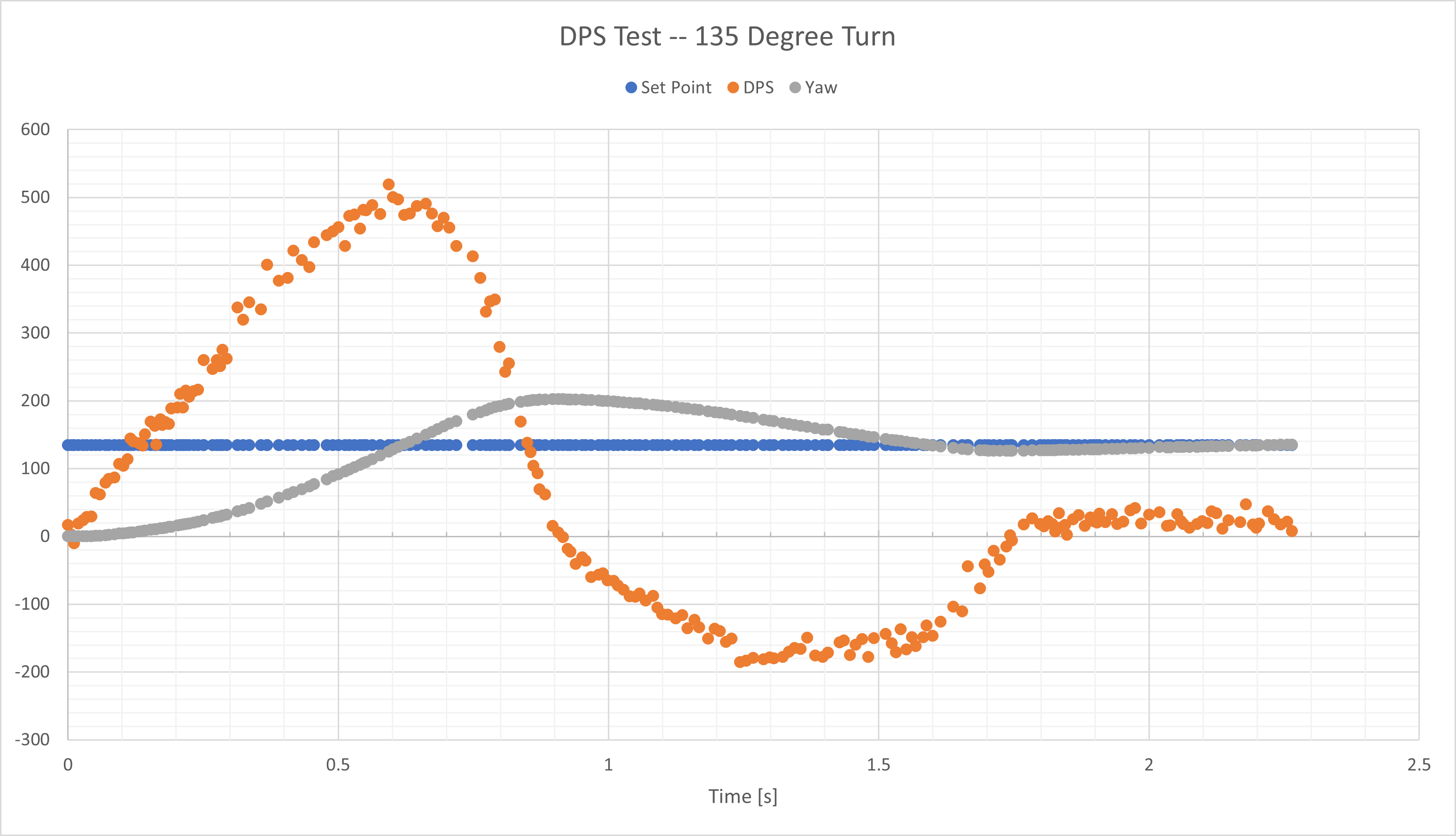
The PID controller was pretty aggressive with the turning, so I decreased the proportional gain to reduce the overshoot that is seen the the DPS Test graph. The turning in the actual run-through had less overshoot. I did a similar test with the speed of the robot and determined 5 seconds was enough time to complete the maximum necessary distances. Since I reduced the proportional gain, I allotted 2 seconds for turns and 5 seconds for the driving portions.
Path Plan
I wrote a python script to calculate all the distances and angles between the waypoints. It also converted the units appropriatly so I could pass parameters to the Artemis via bluetooth and not have to waste time converting units onbaord. I decided to start with the robot oriented at 0 degrees. Then the robot will turn so its facing backwards and drive in reverse towards the first waypoint becuase the walls in the corner are closer and this method is more reliable.
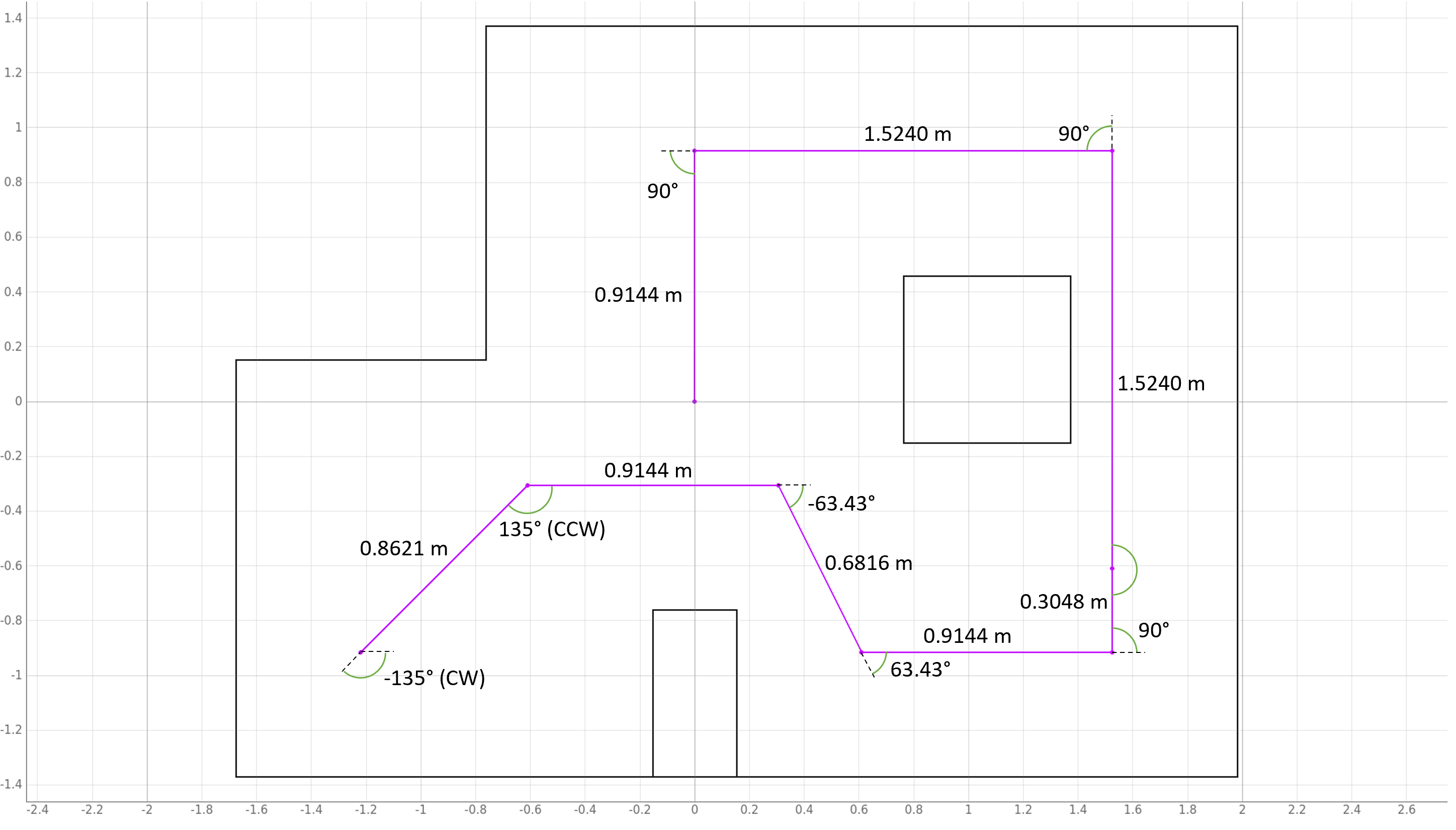
I translated this path plan into a series of commands for the robots to follow. The code also includes the initialization of the objects need for the plotter and localiztion. I had to put in time.sleep() delays in the python script to match the timing in the Artemis code. Without these delays, the script would execute sequentially, but because the commands take time to execute, they wouldn’t actually happen on the real robot. As before, I allotted 2 seconds for turns and 5 seconds for the driving portions.
# Initialize RealRobot with a Commander object to communicate with the plotter process
# and the ArtemisBLEController object to communicate with the real robot
robot = RealRobot(cmdr, ble)
# Initialize mapper
# Requires a VirtualRobot object as a parameter
mapper = Mapper(robot)

# Initialize your BaseLocalization object
# Requires a RealRobot object and a Mapper object as parameters
loc = Localization(robot, mapper)

## Plot Map
cmdr.plot_map()
# Reset Plots
cmdr.reset_plotter()

# Init Uniform Belief
loc.init_grid_beliefs()

--- VISIT WAYPOINTS ---

# pt1 --> pt3
ble.send_command(CMD.TURN, "2.5|0.3|0.3|-135")
time.sleep(2)
ble.send_command(CMD.REVERSE, "45|862.1")
time.sleep(5)
ble.send_command(CMD.TURN, "2.5|0.3|0.3|135")
time.sleep(2)
ble.send_command(CMD.DRIVE, "1.5|0.3|0.3|45|914.4")
time.sleep(5)

# pt3 --> pt5
ble.send_command(CMD.TURN, "2.5|0.3|0.3|-63.43")
time.sleep(2)
ble.send_command(CMD.DRIVE, "1.5|0.3|0.3|45|681.6")
time.sleep(5)
ble.send_command(CMD.TURN, "2.5|0.3|0.3|63.43")
time.sleep(2)
ble.send_command(CMD.DRIVE, "1.5|0.3|0.3|45|914.4")
time.sleep(5)

# pt5 --> pt7
ble.send_command(CMD.TURN, "2.5|0.3|0.3|90")
time.sleep(2)
ble.send_command(CMD.DRIVE, "1.5|0.3|0.3|45|1828.8") # Combine these two segments for time/speed
time.sleep(5)

# pt7 --> pt8
ble.send_command(CMD.TURN, "2.5|0.3|0.3|90")
time.sleep(2)
ble.send_command(CMD.DRIVE, "1.5|0.3|0.3|45|1524")
time.sleep(5)

# pt8 --> pt9
ble.send_command(CMD.TURN, "2.5|0.3|0.3|90")
time.sleep(2)
ble.send_command(CMD.DRIVE, "1.5|0.3|0.3|45|914.4")
time.sleep(5)
-----------------------

# Get Observation Data by executing a 360 degree rotation motion
loc.get_observation_data()

# Run Update Step
loc.update_step()
loc.plot_update_step_data(plot_data=True)
The Run
I got rid of the background noise in the videos, because it was really loud in the lab when I was doing my testing.
Localization
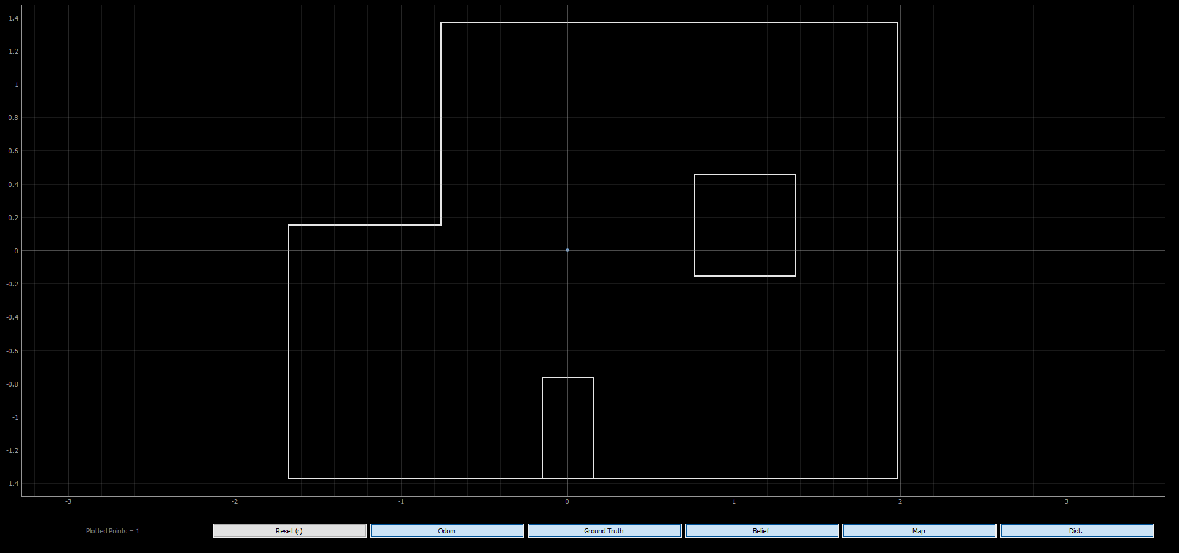
I was able to get the locaization to work well in Lab 12, so I wanted to focus more on executing the navigation in this lab. It would be very simply to implement localization at every waypoint by just calling the same functions I wrote as in Lab 12. That localization data could then be used to inform the controls to adjust the robot’s position. I did perfrom Localization at the last waypoint (0,0) to check that I ended up in the correct place.
Update Step Time: 0.023 secs
Belief: (0.000, 0.000, -90.000)
The x, y, and theta belief of (0 ft, 0 ft, -90.000) was correct! I took this localization data from the more precise, second half of the run, “Segment 2”. In that instance, the robot was mostly in (0,0) tile and was facing downward in the map which would be 270 degrees or -90 degrees.

Discussion
In the full run, I was able to get close to all of the waypoints. However, the robot was not super precise, but the robot was able to get within a tile of the waypoints. The execution wasn’t reliable super either. I started having trouble with the turn at the second waypoint. This was a crucial point, because when the robot overshot the turn, it would skew the enitre rest of the trajectory as errors accumulated throughout the run. I think some of the repeatability was affected by the battery usage.
By breaking up the planned path into two separate runs, you can see that the navigation results were better. The Segment 1 and Segment 2 runs were more precise and reliable, because there was less time for errors to accumulate. I think another method to try to implement to mitigate errors, or migitage the effect of errors, would be to do PID control on the distance from the walls/map boundaries. So instead of doing PID control on the distance traveled and just using the walls as a reference, I would calculate what the distance reading should be from the waypoint to the wall. Then the controls would be more based on the relative position with respect to the walls. This method would place more emphasis on the absolute reading from the ToF data whereas with the method I implemented, it didn’t matter if there was some offset in the ToF data, because I was looking at the change in distance. Overall, I was able to find a solution that was able to perform pretty well.